One of the probe types that can be used with an oscilloscope is a passive-voltage probe. The simplest passive-voltage probe is a coaxial cable. But what happens when a coaxial cable is linked to the device under test? A schematic diagram of the test arrangement is given in Fig. 4.1. The device under test is symbolized as a signal source with an internal source resistance Rs.
For dc voltages, there is no problem as long as R10 Rs, because the part of E appearing at the input of the oscilloscope is
|
Rin E
V osc Rs R1n•
Fig. 4.1
However, in applications involving ac voltages, the stray capacitances have an imperative role. Figure 4.1 shows the signal source loaded by R, n in parallel with Cc + C10• As the impedance Xe of a capacitance is provided by
1
Xe= 2nfC
in which f is the frequency of the ac voltage, a relatively heavier loading of the signal source will occur at higher frequencies.
Example C10 is on the order of 14 to 21 pF; for a coaxial cable of 1-m length, Cc is about 100 pF. At 1 MHz, the impedance of Cc + C10 is approximately1.3 kil. Compared with a R10 of 1 Mil (normally standardized), this means a heavy load.
From this example it will be realized that it is important to measure the voltage at a point in a circuit under test having a low source impedance, in order not to influence the circuit properties too much by the connection of the oscilloscope.
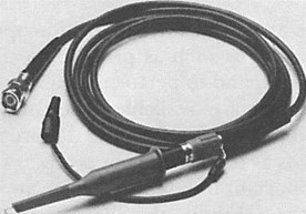
Figure 4.2 shows a typical coaxial cable. On one end, a BNC connector is mounted for connection to the oscilloscope. The other end is provided with a special measuring clip (the probe tip) and a ground lead connector. This type of probe is a 1:1 probe because the signal is not attenuated by the probe. The cable capacitance of this type of probe may be in the order of magnitude like the example.
In cases where the cable capacitance of the l:1 probe will be unacceptable, advantage can be taken of the 10:1 passive probe. Now the signal is attenuated l0 times by the probe. Basically, the object is to create a real IO: l divider for both de and high frequencies. This divider will be independent of the frequency for RC = R1nC1n.
As previously mentioned, C10 can vary from 15 to 25 pF, depending on stray capacitances in the input circuitry of the oscilloscopes, which are different for each instrument. For this reason, C is made variable.
However, a more realistic schematic diagram would show that the compensation is for 120 pF, giving a value of C = 13 pF. At the probe tip, there should also be a stray capacitance C. of about 2 to 4 pF from the tip itself to its environment. Effectively, a complete load capacitance of C8 parallel to C and Cc + C10 in series would be obtained, resulting in about 15 pF. But 15 pF is far less than 120 pF. A disadvantage might be that the signal is attenuated 10 times at the input of the oscilloscope.